
 This project has received funding from
the European Union's
This project has received funding from
the European Union's 
Signal in a ZULF NMR Experiment: Getting the biggest bang for your buck
In the two previous blogposts we have talked about the ZULF-NMR experiment and how we obtain the signal from our sample. But how good or useful is this magnetic field emanating from the sample that we wish to study? Well, it is only valuable insofar as we can discern the signal from the background noise (which is unavoidable in any real experiment). For this reason, we tend to talk about signal-to-noise ratio (SNR or S/N) rather than referring to the signal on its own.
There exists a plethora of ways that noise can meddle in our experiments to obscure the signal – some of which are illustrated in Fig. 1. We can suffer from vibrational noise coming from mechanical vibrations of the table on which the experimental setup rests, and ambient light from the surroundings can be picked by the photodetector (at the end of the day, these are basically tiny cameras that we don't want saturated). Important also is the laser system mentioned in Blog Post 2: any instability in the frequency or intensity of the laser beam generates noise. Even sound – which induces pressure variations in the air through which our laser beams propagate – can ever-so-slightly change the light path and therefore introduce noise.
One must also consider noise coming from the electronics in our setup. Random thermal currents in the mu-metal shield produce a type of noise called Johnson-Nyquist noise. There is also noise that comes from the mains power (i.e., the wall electricity plugs) at either 50 or 60 Hz (depending on your continent) and at the overtones thereof.
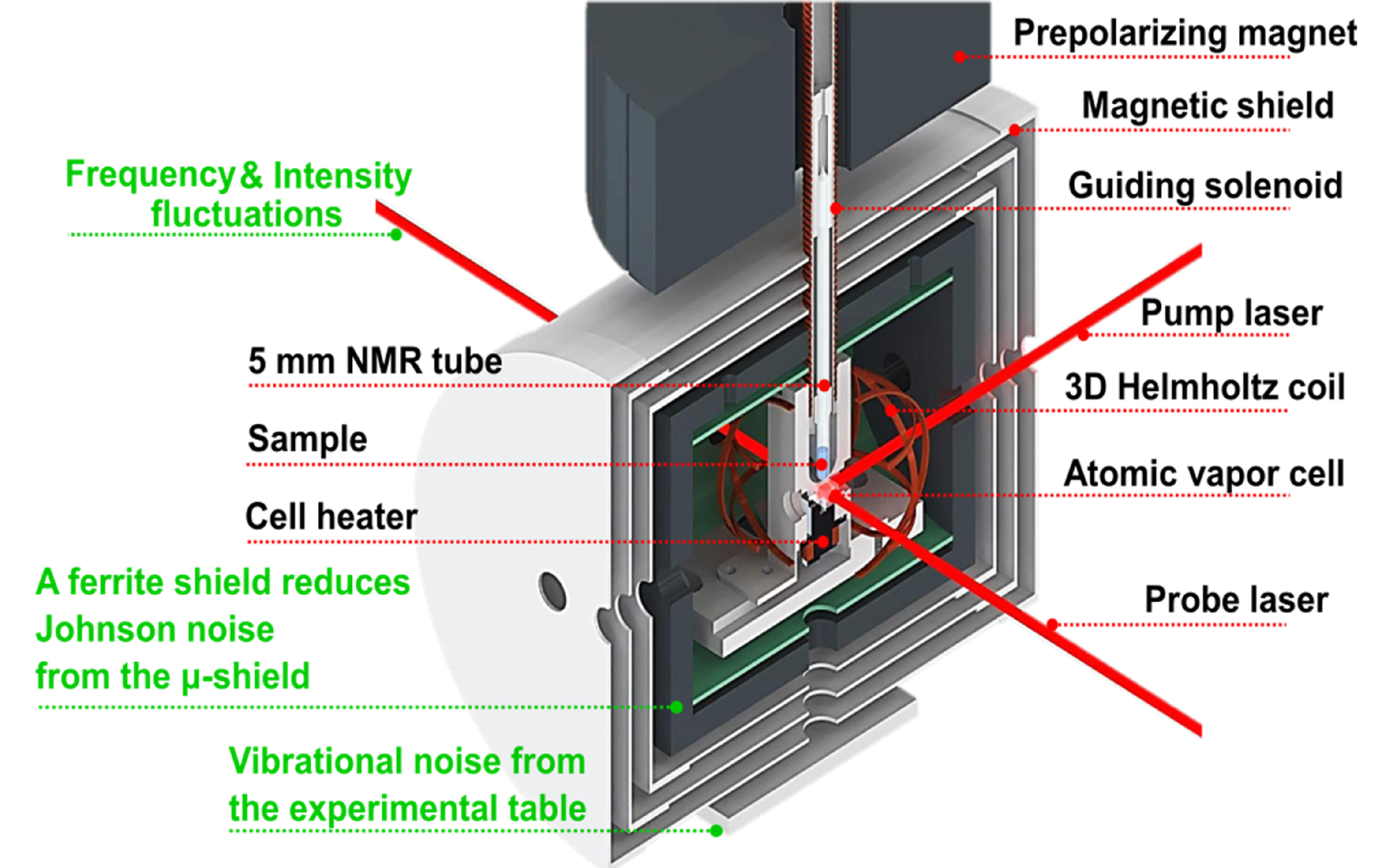
Figure 1: Different components of the ZULF-NMR experiment (black text) and possible noise sources / measures against noise (green text), adapted from [1].
To make things worse, there even exists noise due to the quantum features of nature itself! Examples include the so-called photon noise and spin-projection noise, consequences of such fundamental quantum laws as the Heisenberg uncertainty principle – crazy stuff.
Nonetheless, there is some good news: these sources of noise are different and therefore generally behave differently from our signals.
For example, some electronic noise sources have a characteristic inverse dependence on frequency (f), frequently called 1/f or pink noise
.
Because of this distinguishability we can develop different strategies to fight against certain type of noise. Are we disturbed by ambient light and sound?
Let's enclose the setup in a dark box with insulating foam (see Fig. 2). Vibrational noise is an issue? Let's rest the setup on sorbothane sheets,
a type of material that absorbs vibrations, and make extra sure that all of the optical components are rigidly held in place.
For other noise sources more elegant approaches can be taken. We can replace the innermost layer of the mu-metal magnetic shield with a ferrite layer, which is electrically insulating, in order to reduce Johnson-Nyquist noise. If the laser intensity fluctuates, is it possible to stabilize it using a feedback loop implemented via, for example, an acousto-optic modulator (AOM). An AOM shifts the frequency and power of the laser light using sound waves. One of the branches of the light diffracted by the AOM can be detected with a photodiode and fed into a PID-control system. By doing this a closed loop is built that serves to stabilize the intensity of the light beam.
Since the bandwidth of our experiment is low (typically <1 kHz), we are especially affected by low-frequency electronic noise. We can fight against it using a creative idea: we use a photoelastic modulator (PEM) to transfer the signal into the high-frequency regime (e.g. 50 kHz), where that noise is smaller. We then use a lock-in amplifier to demodulate the signal back to the low-frequency regime, hence retrieving the signal in its appropriate frequency range. Is it important to note that the previous scheme cannot prevent magnetic-field noise, which is a flowing current picked up somewhere in the setup that generates a real magnetic field.
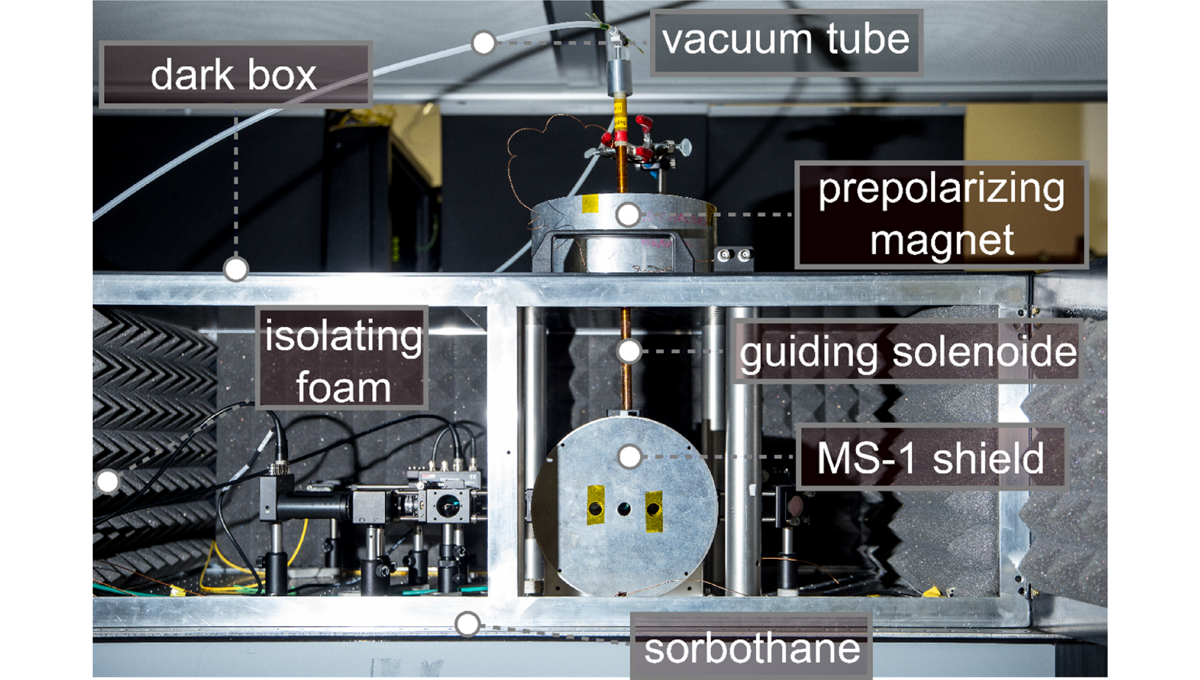
Figure 2: ZULF-NMR spectrometer where isolated foam and a dark box where used to reduce noise due to ambient light and sound.
We still must mention a very important concept: common-mode noise. In simple terms, this refers to any noise which is the same (common) in different measurement channels. While the idea of having a noise source that affects everything might sound horrifying, it’s actually a scenario that is easy to deal with: we simply need measure in two different volumes, and take the difference between these measurements. Provided that the signal is not the same in both channels, we have eliminated the common-mode noise while retaining our signal.
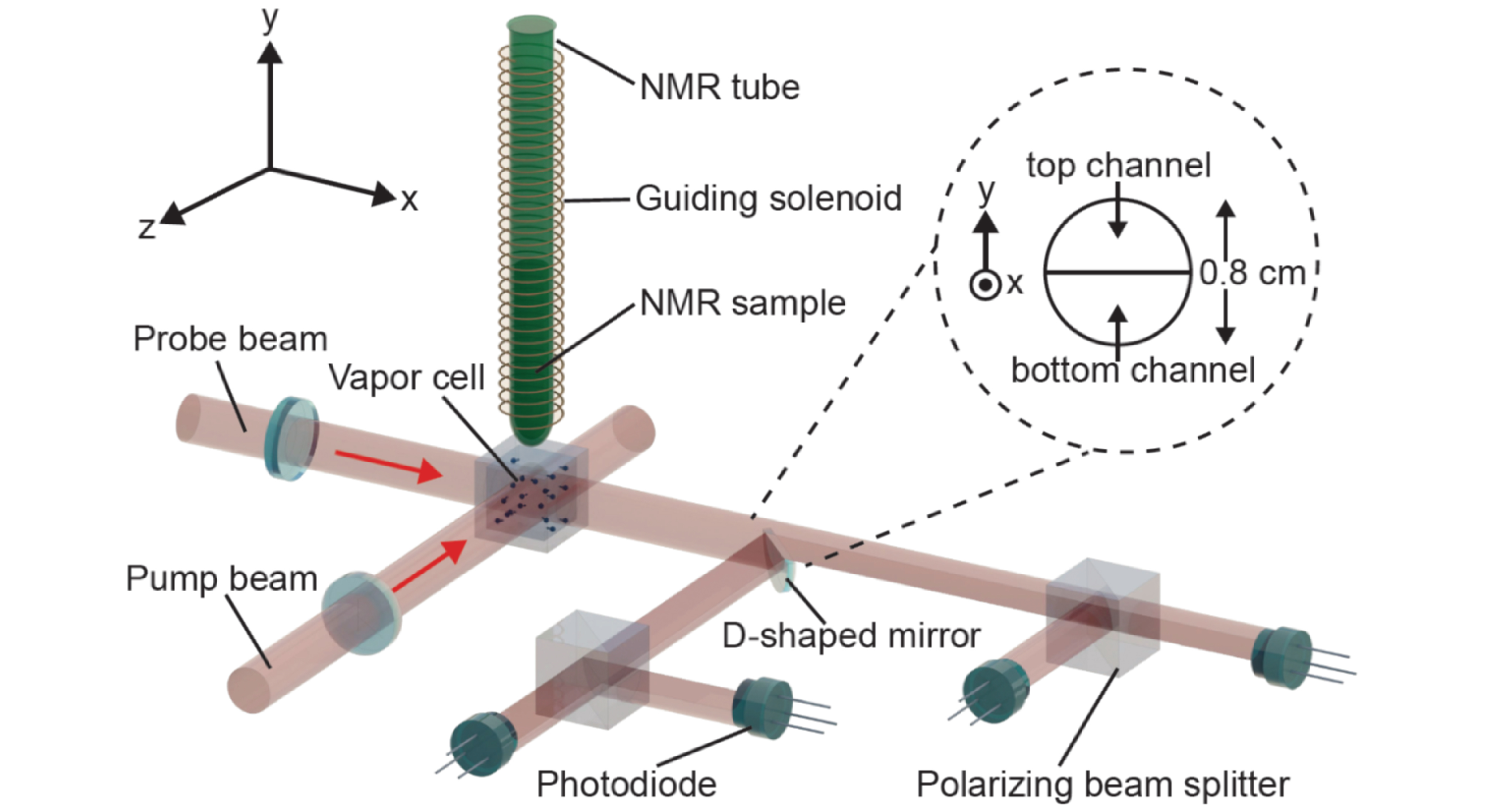
Figure 3: Gradiometer achieved by the difference of a "top" magnetometer and a "bottom" magnetometer defined by their spatial separation. The key is that the Rb atoms in the top half of the vapor cell sense a higher NMR signal than the atoms in the bottom half, but the common-mode noise is the same in both channels. Image reproduced from Ref. [3].
One notable example is that rather than measuring magnetic field with a single magnetometer, we can measure the gradient of magnetic field with a gradiometer. Fig. 3 shows how a D-shaped mirror can be implemented in the optical system to separate the signal based on distance to the NMR tube, which is a simple gradiometer.
The reason the gradiometer scheme works is because the signal is larger closer to the sample, but many noise sources are the same in both channels. This is an example of arranging our sensors to maximize the signal we are detecting. To do this, we had to previously understand how our noise and signal profiles look like. If we imagine our sample as a uniformly-polarized sphere, the magnetic-field signal can be easily written down as that of a dipole field, so we can arrange the detectors in a smart way to optimize the signal we measure. For non-spherical samples, geometric demagnetization effects from the shape of the sample and detector can lead to no observable signal being picked up. Fig. 4 illustrates three extreme cases in which no signal would be detected: detection (a) in the middle of a uniform bath of polarized dipoles; (b) next to an infinitely large plane of dipoles oriented normal to the plane; (c) outside an infinitely long tube of dipoles oriented in the long axis. This last is example is not so intuitive as the others, but one way to imagine the problem is to think of a perfect toroidal solenoid. This produces no magnetic field outside the toroid, since the field lines can converge inside. Now imagine that the toroid is increased in diameter until it is, to the observer, more-or-less an infinitely long, straight solenoid. Et voilà – no field outside!
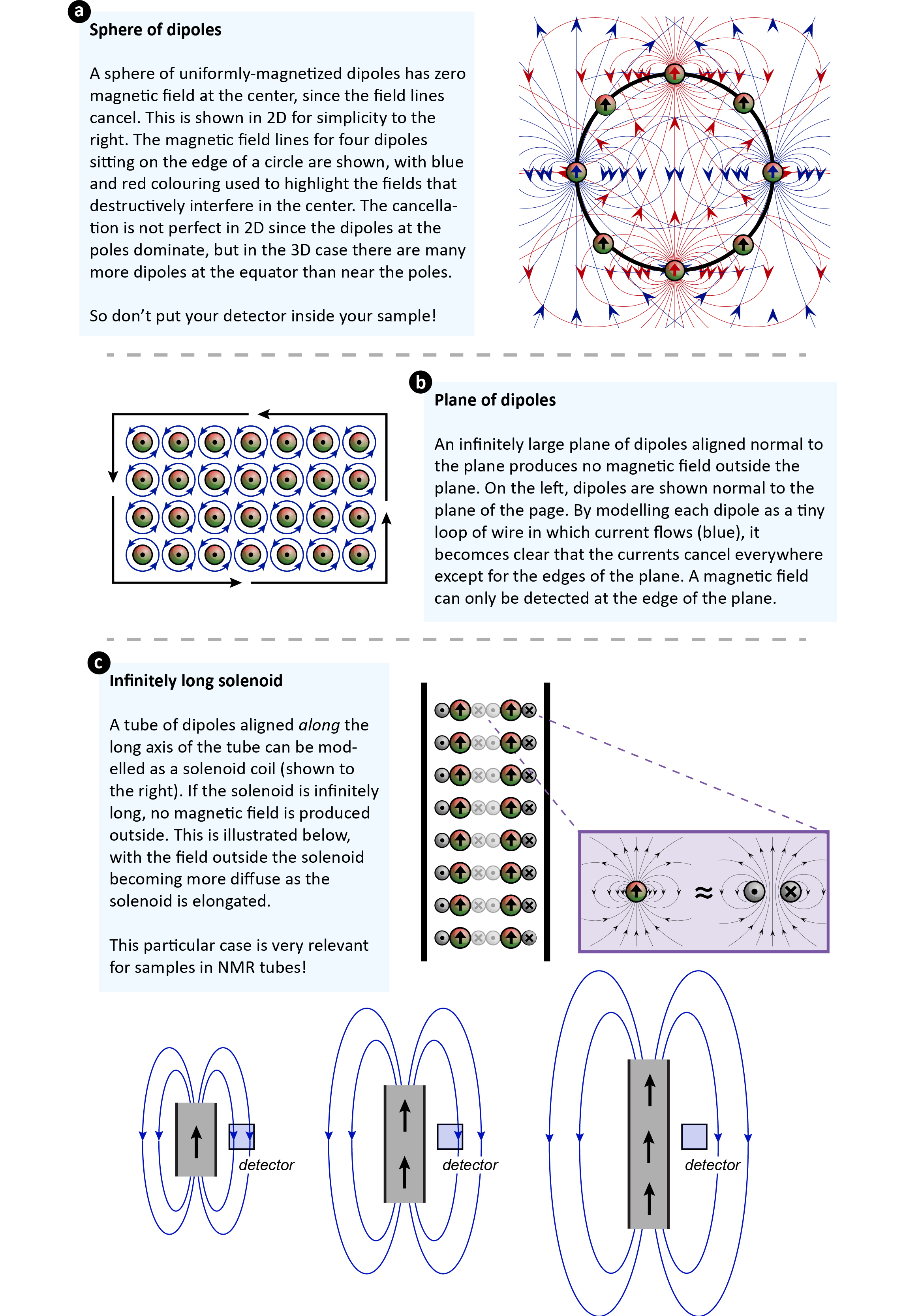
Figure 4
Understanding the geometry between the signal emanating from the sample and the placement of the detector is of paramount importance for maximizing the
signal – the so-called filling factor
in NMR literature – and avoiding accidentally detecting nothing. If we detect from underneath an NMR tube,
the sample can be modelled to a good approximation as a magnetized sphere. If we detect from the side of an NMR tube with a larger sample volume,
it can be modelled as a magnetized cylinder. As an example of good geometries, in reference [4] an NMR signal, thought of as magnetized cylinder,
is detected from the sides using two Rb vapor cells in a gradiometer configuration.
High-field NMR operates at radio frequencies, and uses inductive detection, which means noise is mostly Johnson-Nyquist noise from the probe circuitry [5]. ZULF NMR is a different animal, which operates at low frequencies and uses optically-pumped magnetometer detection, so totally different considerations are needed to minimize noise and optimize detection sensitivity. It is easy to find oneself overwhelmed by the long list of possible noise sources, but there is no need to panic! It is simply important to understand your experimental setup and deal with noise issues one by one: Find the noise source that limits your overall sensitivity, and tackle this first. Then move on to the next biggest source. By doing this, we are moving towards some exciting applications of ZULF NMR! With sensitivity as good as a couple fT/√Hz, we can use ZULF-NMR to expand the boundaries of physics by probing exotic spin interactions and even search for dark matter (DM), one of the biggest unanswered mysteries of modern science.
-Stay tuned-
Román Picazo-Frutos
I am a PhD student in the Budker group in the Helmholtz-Institute Mainz. I am interested in hyperpolarization, atomic physics, photonics and relaxometry in NMR. I am looking forward to expanding the applications of ZULF NMR and collaborating with scientists with similar interests.
Literature references:
- Jiang, M.; Wu, T.; Blanchard, J. W.; Feng, G.; Peng, X.; & Budker, D. Experimental benchmarking of quantum control in zero-field nuclear magnetic resonance, Sci. Adv. 2018, 4(6), 6327
- Chatzidrosos, G.; Wickenbrock, A.; Bougas, L.; Leefer, N.; Wu, T.; Jensen, K.; Dumeige, Y.; Budker, D. Miniature cavity-enhanced diamond magnetometer, Phys. Rev. Appl. 2017, 8, 044019
- Jiang, M.; Frutos, R. P.; Wu, T.; Blanchard, J. W.; Peng, X.; Budker, D. Magnetic Gradiometer for the Detection of Zero-to Ultralow-Field Nuclear Magnetic Resonance. Phys. Rev. Appl. 2019, 11(2), 024005
- Xu, S.; Rochester, S. M.; Yashchuk, V. V.; Donaldson, M. H.; Budker, D. Construction and applications of an atomic magnetic gradiometer based on nonlinear magneto-optical rotation. Rev. Sci. Instr. 2016, 77(8), 083106
- Hoult, D. I.; Richards, R. E. The signal-to-noise ratio of the nuclear magnetic resonance experiment. J. Magn. Reson. 1976, 24(1), 71-85